In the early 14th century, an English philosopher known as William of Ockham spoke thus: “pluralitas non est ponenda sine necessitate.” Centuries later the credo entities should not be multiplied without necessity has grown to be a universal principle, known as the principle of parsimony, which systematically biases decision making across the vast and varied scientific landscape. My introduction to this principle came during a statistics class when a senior student advised me that if I mention parsimony the department statisticians will do a little dance and award me an entire point on my assignment! Considering my main objective in life was to inflate my GPA, parsimony held a clear value. I’ve since graduated and parsimony has lost its point awarding abilities. Disappointingly, it also seems to have little effect on my supervisor’s dance tendencies. So, if parsimony cannot promote my personal goals, what is parsimony worth?
Parsimony in knowledge discovery
The definition of parsimony is by itself non-contentious to anyone who isn’t an avid supporter of redundancy. It also isn’t useful given that its value is context dependent. My interest lies in the domain of knowledge discovery and therefore this is the context in which parsimony will be evaluated. Let’s break down the definition and embed it into context: entities should not be multiplied without necessity. Our ultimate goal is to justify the should not part, that is to identify the utility of simplicity. To do this we first need to define the necessity. For without a target, we cannot judge when the “multiplication of entities” has to cease. Say we want to explain why people with sleep problems also experience fatigue and irritability. After we search for possible explanations, we want to select one—the best one ideally. So we need to compare our explanations, which means we need to transform them into something we can compare in terms of both accuracy and simplicity. One way to do this, is to express our theories as models and use some quantitative metric that reflects the extent to which they fit with our observations (e.g. the bayesian information criterion). We can call this model fit. Drawing from our example we can manufacture two quick-and-dirty theories: a) reciprocal causal associations between all three symptoms explain their co-occurrence; or, more “simply” b) a fourth variable (e.g., depression) causes all of them, which is why they co-occur. These explanations result in two models with different numbers of parameters. We can use the number of parameters needed to formalize an explanation to approximate its simplicity. Thus, we redefine our entities as the number of parameters needed to specify a given explanation. In the case that our models have the same fit, parsimony would dictate that we choose the simpler of the two—the more parsimonious model. Indeed, many metrics of model fit have an inbuilt penalty for the number of parameters a model has, making model fit the product of a trade-off between complexity and fit to the data1. The principle of parsimony can now be rephrased as: the number of parameters should not be multiplied further than is necessary to improve model fit. This brings us to the crux of the matter—why is this a good idea?
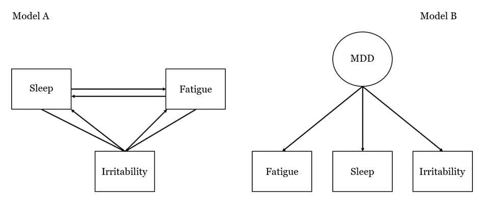
Figure 1. Schematic of two example models one complex (Model A) and one simple (Model B)
Parsimony as bias
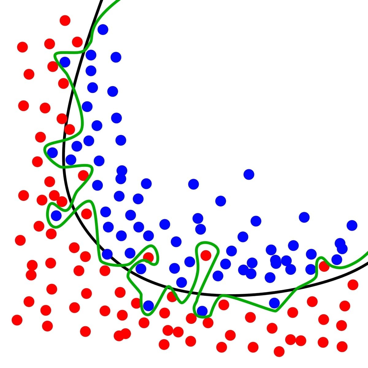
Ideally, we want a model that fits both to our current observations but also fits well to independent samples. Otherwise, we run the risk of a model that fits tightly to random fluctuations in our data outperforming a model that better approximates the process of interest. This is commonly known as overfitting and is problematic since most real-world data reflects both the process of interest and sample-specific noise. To mitigate overfitting one can look at the generalization error, which indicates how well a model performs in a previously unseen sample. The rationale being that if a model performs well on a given dataset because it fits well to the sample-specific noise, then it should do poorly when fitted to another sample. While a model that fits well to the process of interest should fit well to all samples that appropriately measure that process. A common justification for choosing the most parsimonious model is that it will always minimize generalization error. Which brings us to a popular definition of parsimony: the simpler of two models with equal fit on a given dataset, will fit better on unseen datasets. This statement when taken literally is false. The falsity of this statement follows from David Wolpert’s “no free lunch” theorem2. What the “no free lunch” theorem shows is that for any pair of models there are as many domains where the simpler model is preferable as there are domains where the more complex model is preferable. This essentially invalidates the universality of simplicity as a guiding tool for model selection—in fact for any two models A and B there are as many domains where model A has lower generalization error as there are domains where this is true for model B. The more interesting question, however, isn’t whether parsimony guarantees lower generalization error. What is practically interesting is whether the use of parsimony will lead to lower generalization error in most (or all) applied situations. Domingos follows this precise question in an extensive review of empirical circumstances that contradict this weaker justification for parsimony3. Specifically, he shows that within the domain of machine learning simpler models often lead to higher generalization error. Therefore, both empirically and mathematically the claim that parsimony leads to lower generalization error is found wanting.
Simplicity and comprehensibility
So what if parsimony doesn’t buy us more accurate predictions? Arguably a worthwhile cost if our main aim is to understand the world and simpler models are easier to comprehend. But what makes a model more comprehensible? In 2006, van der Maas and colleagues, debuted their theoretical alternative to the dominant g-factor model that presented a single entity as the causal driver of intelligence—much like our fictitious model B (Figure 1). The mutualism model, as van der Maas termed it, is much more complex in terms of parameters than the g-factor model and fits just as well to cross-sectional observations. If we use comprehensibility as a tie-breaker we should be safe betting on the more parsimonious model. Not so fast. Simplicity in terms of the effective number of parameters needed to specify the g-factor model does not reflect its comprehensibility. As van der Maas argues, the mutualism model certainly can multiply the number of parameters, but the g-factor model conjures up “a rather mysterious” hidden variable4. The same can be said for our toy models. Model B buys its simplicity by manufacturing an entirely new, arguably opaque entity, while model A presents a more complex mechanism that nevertheless is easier to comprehend. In other words, we can better intuit how sleeplessness might make one tired and therefore irritable, while it is harder to parse what this depression variable actually is and how it brings symptoms to be. It seems that parsimony also fails to guarantee superior comprehensibility in some domains.
Parsimony in model search
It seems not even parsimony suffices as a fast-and-hard rule that we can generously apply to any domain of science. But there is one domain where parsimony may still be unequivocally welcome. This is the domain of model search. Blumer showed mathematically that the more models we test on our data, the greater the chance that the best fitting model will fit poorly on other samples5. This is essentially multiple testing in model search and reflects the fact that testing more models increases the probability that we find a good fitting model purely by chance.
Domingos presents an accessible overview of the mathematical argumentation in his review. It goes something like this. Let’s say that the generalization error of a hypothesis is greater than ε. From this it follows that the probability that our hypothesis is correct on x number of independent samples is smaller than (1 — ε)x[^ refers to the power of, e.g. 2^2 = 4. Our cutting-edge editor does not have superscript functionality.]. If we consider n number of hypotheses then the probability that at least one of them is correct in all x independent samples is n(1 — ε)^x. If we substitute this with real numbers, we can see that the probability of at least one of our hypotheses being correct increases with the number of hypotheses considered. That is 2(1 — 4)^2 is 18, which is smaller than 4(1 — 4)^2 which is 36. In a nutshell6, “if we select a sufficiently small set of models prior to looking at the data, and by good fortune one of those models closely agrees with the data, we can be confident that it will also do well on future data.7” Hence, multiple testing provides a safe-haven for the historic concept of parsimony, but veers from the traditional interpretation of parsimony as it pertains to the assumptions within an explanation.
Goodbye parsimony
Throughout my reading for this blog, I had to bury my naive belief in the powers of parsimony. That’s strike two. Now I will be forced to constrain my models in another way. Through the grind of gaining domain knowledge and thoughtfully integrating it into the a priori specification of my models. This currently seems like the only effective recourse to reduce the number of models tested and improve comprehensibility. Thanks for the points parsimony, you’ve gotten me this far…
Author: Michael Aristodemou
This can lead to situations where parsimony leads us to choose the simpler model with worse fit to the data. Meaning parsimony is not just a tie-breaker.↩︎
Wolpert, D. H. (1996). The lack of a priori distinctions between learning algorithms. Neural computation, 8(7), 1341-1390.↩︎
Wolpert, D. H. (1996). The lack of a priori distinctions between learning algorithms. Neural computation, 8(7), 1341-1390.↩︎
Van Der Maas, H. L., Dolan, C. V., Grasman, R. P., Wicherts, J. M., Huizenga, H. M., & Raijmakers, M. E. (2006). A dynamical model of general intelligence: the positive manifold of intelligence by mutualism. Psychological review, 113(4), 842.↩︎
Blumer, A., Ehrenfeucht, A., Haussler, D., & Warmuth, M. K. (1987). Occam’s razor. Information Processing Letters, 24, 377(380).↩︎
Wolpert, D. H. (1996). The lack of a priori distinctions between learning algorithms. Neural computation, 8(7), 1341-1390.↩︎
Wolpert, D. H. (1996). The lack of a priori distinctions between learning algorithms. Neural computation, 8(7), 1341-1390.↩︎